Demographic Characters and Access to Public Transit in Greater Vancouver: Machine Learning Modeling
A shorter high-level summary of the project can be found here. For an interactive web application with simulation results of priority neighborhoods, see here.
This is part 3 of a series of in-depth posts about this project including
For the Jupyter Notebook with full analysIs, please see here. The GitHub repo of this analysis is located here.
Remove extreme observations
Now that we have tabular data of demographic characters, transit access and transit usage down to the DA level, I will pre-process the data so that it is ready to be put into machine learning algorithms. Firstly, features with all NA data are removed (in fact there are two such features). Then, I will remove rows that have irregular, or extreme values for important variables, as shown in the following table:
| Removal Criteria | Number of DAs removed |
|---|---|
| DAs with zero population in 2016 | 8 |
| DAs with zero land size in 2016 | 1 |
| DAs with with land size 2 standard deviations above the mean | 8 |
| DAs with with population density 2 standard deviations above the mean | 37 |
| DAs with with population density 2 standard deviations below the mean | 165 |
| DAs without transit service or stops in the neighborhood area | 49 |
| DAs whose proportions of residents using transit are invalid (NAs) | 2 |
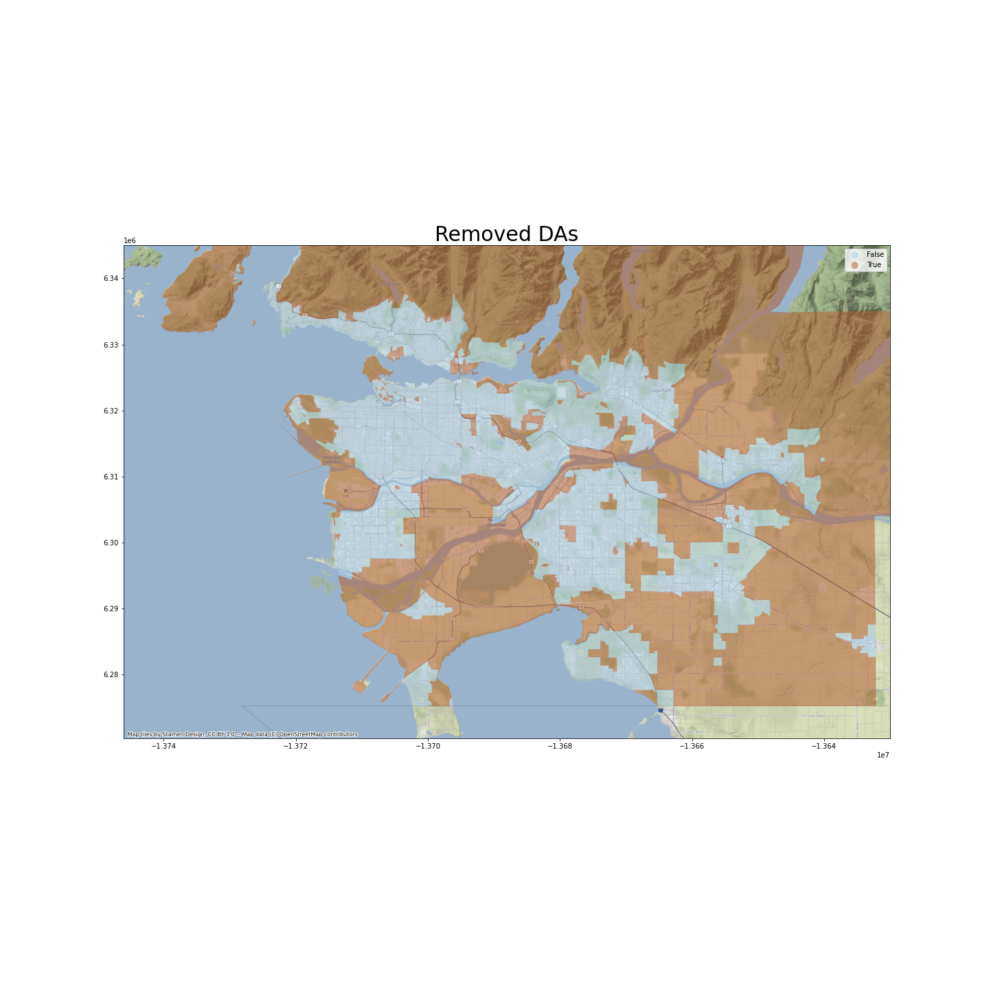
The following map shows in brown DAs that have been removed from our next steps of analysis.

Feature engineering of census data
Most explanatory variables of this study come from the 2016 census, except for two, namely the number of transit services in the neighborhood area per person, and the number of transit stops in the neighborhood area per person, which are from the GTFS Data. I have also calculated some proportional relationships between census variables and added them to our analyses, and removed some confounding variables.
Create proportional variables
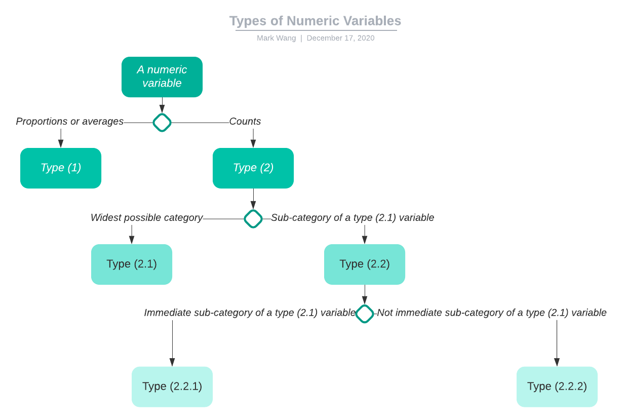
Proportional variables are calculated based on numeric features in the census data. There are two types of numeric columns:
-
(1) Proportions or averages. An example of proportion is “Population density, per square kilometer”, and an example of average is “Average Household Size.”
-
(2) Counts. Most numeric variables are in this category, for example (number of) “Private households”.
We will put type (1) variables directly into our models. For type (2) variables, I divide them into two sub-types:
- (2.1) Counts of subjects belonging to the widest possible category in a DA, for example, total number of people who are immigrants.
We will put type (2.1) variables directly into our models.
-
(2.2) Counts of subjects belonging to a sub-category of a type (2.1) variable in a DA. There are further two sub-types:
-
(2.2.1) Counts of subjects belonging to an immediate sub-category of a type (2.1) variable, for example, total number of immigrants who are born in Asia.
We will use type (2.2.1) variables in two ways. Firstly, we will put them directly into our models. Secondly, we will calculate the proportion of each type (2.2.1) variable to the type (2.1) variable that it belongs to.
- (2.2.2) Counts of subjects belonging to a further-off sub-category of a type (2.1) variable, for example, total number of immigrants who are born in India, Asia.
We will use type (2.2.2) variables in three ways. Firstly, we will put them directly into our models. Secondly, we will calculate the proportion of each type (2.2.2) variable to the type (2.1) variable that it ultimately (but not immediately, by definition) belongs to. Thirdly, we will calculate the proportion of each type (2.2.2) variable to the type (2.2.1) or type (2.2.2) variable that it immediately belongs to.
The following chart explains types of numeric variables.

Remove confounding variables
I have also removed variables that sit on the causal chain from access to transit to proportion of transit use. Such variables, theoretically, are impacted by the access to public transportation, and can in turn impact the use of public transportation. Confounding variables include:
- Mode of Commuting
- Duration of Commuting
- Time of the day when leaving for work
In total, 572 new proportional variables have been created, and 76 confounding variables have been excluded.
Create train and test splits
There are 2544 observations in the train split and 636 observations in the test set.
Preliminary analyses
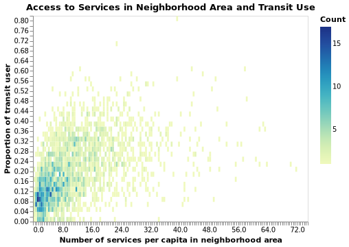
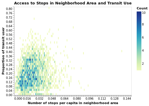
Before stepping into modeling, I did some quick sanity check on the correlation between access to, and public usage of, transit across DAs in GVA. The two plots below show that their relationships seem to be positive, which is expected.


Modeling
Model selection and hyperparameter tuning
I selected three models, namely (1) dummy regression, (2) LASSO, and (3) Random Forest regression.
- Dummy regression
The dummy regression model has both training and testing R-squared close to zero, which is expected.
- LASSO regression
I tuned the alpha hyperparameter in the model using grid search. As shown in the table below, an alpha value of 0.0001 turns out to be the best.
| Validation score rank | Mean validation R-squared | Alpha hyperparameter | Mean Fit Time |
|---|---|---|---|
| 1 | 0.680 | 1.00E-04 | 13.815 |
| 2 | 0.651 | 1.00E-03 | 19.746 |
| 3 | 0.627 | 1.00E-05 | 14.588 |
| 4 | 0.518 | 1.00E-02 | 21.070 |
| 5 | 0.354 | 1.00E-01 | 14.889 |
| 6 | 0.255 | 1.00E+00 | 2.017 |
| 7 | 0.113 | 1.00E+01 | 1.835 |
| 8 | -0.001 | 1.00E+02 | 1.322 |
| 9 | -0.001 | 1.00E+03 | 1.279 |
| 9 | -0.001 | 1.00E+04 | 1.002 |
- Random Forest model
I tuned max_depth, max_features, min_samples_leaf, min_samples_split, and n_estimators hyperparameters using randomized search. The table below shows the best combination of hyperparameters.
| Validation score rank | Mean validation R-squared | Max_depth hyperparameter | Max_features hyperparameter | Min_samples_leaf hyperparameter | Min_samples_split hyperparameter | N_estimators hyperparameter | Mean Fit Time |
|---|---|---|---|---|---|---|---|
| 1 | 0.6760 | 100 | auto | 2 | 5 | 2000 | 1401.222 |
| 2 | 0.6759 | 100 | auto | 1 | 5 | 200 | 142.685 |
| 3 | 0.6755 | 40 | auto | 1 | 2 | 200 | 155.870 |
| 4 | 0.6751 | 40 | auto | 2 | 10 | 600 | 336.548 |
| 5 | 0.6745 | 100 | auto | 2 | 10 | 2000 | 1302.495 |
| 6 | 0.6720 | 40 | auto | 1 | 5 | 200 | 144.661 |
| 7 | 0.6657 | sqrt | 2 | 2 | 200 | 5.166 | |
| 8 | 0.6642 | 100 | sqrt | 1 | 10 | 2000 | 45.181 |
| 9 | 0.6639 | 100 | sqrt | 4 | 2 | 2000 | 42.367 |
| 10 | 0.6630 | 10 | sqrt | 2 | 5 | 600 | 12.829 |
Model evaluation
After hyperparameter tuning, I compared the performance, as measured by root mean squared error (RMSE), among the three models on the whole train split. Random forest regression seems to perform the best among the three models.
| Model | Train Split RMSE |
|---|---|
| Dummy Model | 0.120 |
| LASSO Regression | 0.054 |
| Random Forest Regression | 0.027 |
I then fitted the best Random Forest model with the test split, and got a RMSE of about 0.070.

