Demographic Characteristics and Access to Public Transit in Greater Vancouver: Analyses and Recommendations
A shorter high-level summary of the project can be found here. For an interactive web application with simulation results of priority neighborhoods, see here.
This is part 4 of a series of in-depth posts about this project including
For the Jupyter Notebook with full analysIs, please see here. The GitHub repo of this analysis is located here.
Where should transit infrastructure development take place in the Greater Vancouver Area?
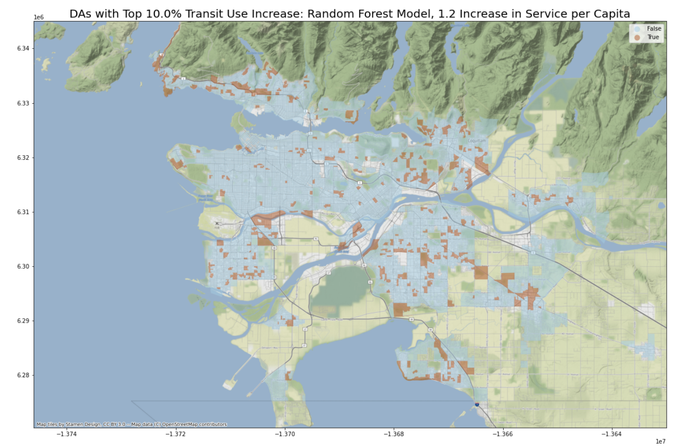
In order to understand where Greater Vancouver Area’s public transit agency should invest in infrastructure development, I try to identify places in the region where the same increase in access to transit service will lead to the most increase in transit use. Using the 2016 Canadian census data and the GTFS dataset, I am able to build two machine learning models: LASSO regression and Random Forest. After training our models with the real dataset, I tweaked the input data a little bit to simulate scenarios where access to public transit is marginally increased across the Greater Vancouver Area. It turns out the following areas will benefit the most, as measured by public transportation use:
-
The downtown core: Yaletown and areas around the Waterfront
-
North Vancouver and West Vancouver: neighborhoods close to the Trans-Canadian Highway
-
Richmond: areas on the north and south edges
-
Burnaby: areas further off from the Trans-Canadian Highway
-
Surrey: areas in the southwest and northeast
Model Diagnostics
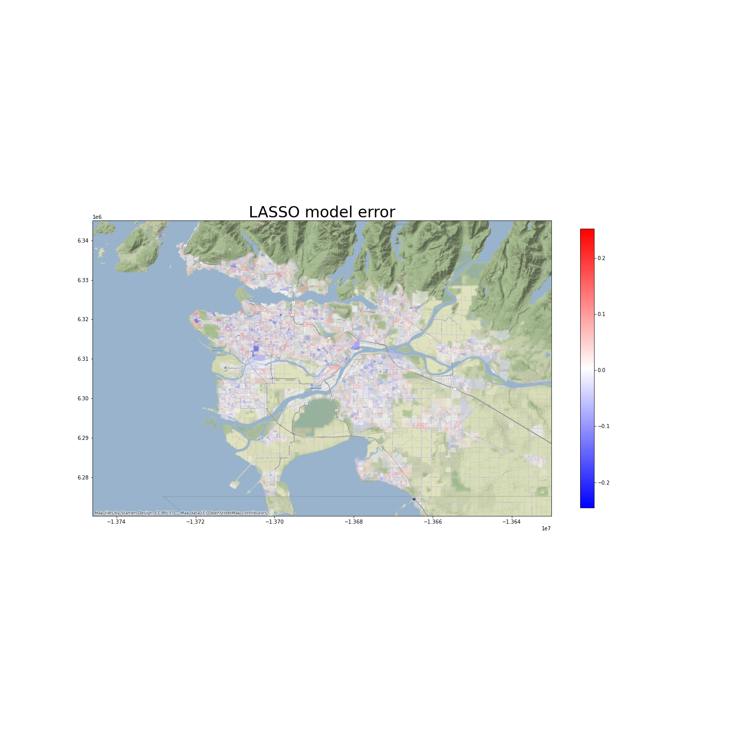
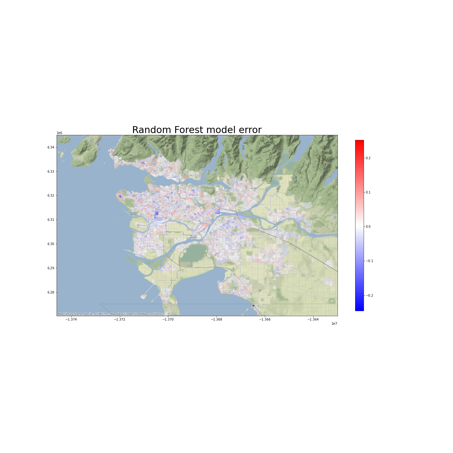
Before drawing conclusions from our models, we want to examine whether there is spatial auto-correlation of their prediction errors. We believe that the higher the spatial auto-correlations are, the more unexplained factors, which affect transit use and are spatially clustered, there will be. Therefore, we want to see less, and ideally no spatial auto-correlation.
As shown in the maps below, the spatial-autocorrelation problem does not seem to be severe. Indeed, the Moran’s I is 0.05 for the LASSO model, and 0.18 for the random forest model. However, p-tests show that we do have spatial-autocorrelation problems, at confidence levels of 0.001.
Model analyses: feature importance
Both LASSO and Random Forest models give easy access to measurements of global feature importance. For the LASSO model, I use the magnificence of coefficients to roughly estimate each variable’s importance. For the Random Forest model, I use the impurity measurement of each variable’s importance, and calculate SHAP (SHapley Additive exPlanations) values.
In addition, the three types of input variables, namely categorical_features, numeric_features, and proportion_features are scaled differently in the preprocessing step. Therefore, I will review the important variables for all three categories separately.
Categorical features
LASSO model
The table below shows the five categorical features that mostly strongly predict high proportion of transit use among residents. They are ADA or CCS areas.
| feature | coeffs | |
|---|---|---|
| 148 | ADAUID_59150117 | 0.097663 |
| 7 | CCSUID_5915022 | 0.069961 |
| 8 | CCSUID_5915025 | 0.065468 |
| 138 | ADAUID_59150107 | 0.053888 |
| 114 | ADAUID_59150082 | 0.048754 |
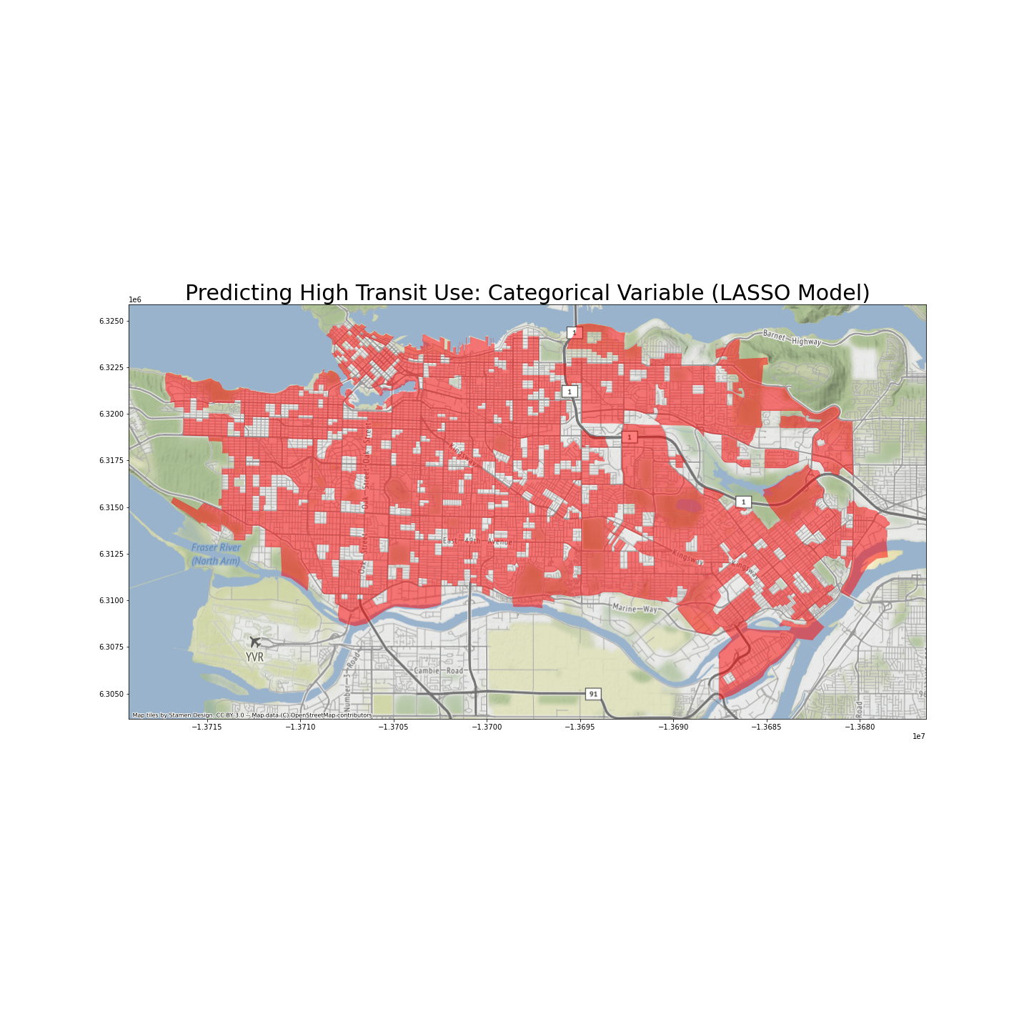
As shown in the map above, areas in the city of Vancouver tend to have high proportions of people using public transit.
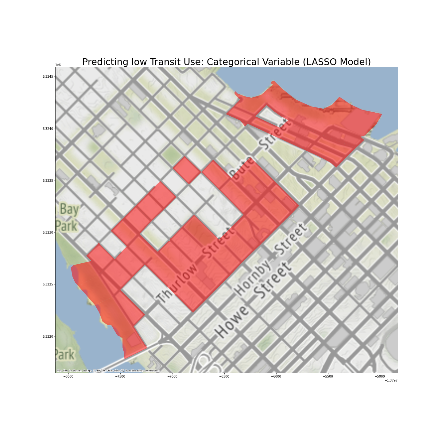
Somehow unexpectedly, regions that most strongly predict low public transit use are also in the downtown area, distributed along Thurlow Street. They are also in the CCS which predicts high transit use. In other words, these areas may have lower transit use than their immediate neighbors, but not necessarily compared to other ares in GVA.
Random Forest model
The table below shows the five categorical features that most strongly impact proportion of transit use among residents. They are CSD or CCS areas. We cannot know the direction of impact from these impurity measures.
| feature | impurity_importance | |
|---|---|---|
| 18 | CSDUID_5915022 | 0.008434 |
| 8 | CCSUID_5915025 | 0.005865 |
| 2 | CCSUID_5915001 | 0.004445 |
| 7 | CCSUID_5915022 | 0.003664 |
| 148 | ADAUID_59150117 | 0.001297 |
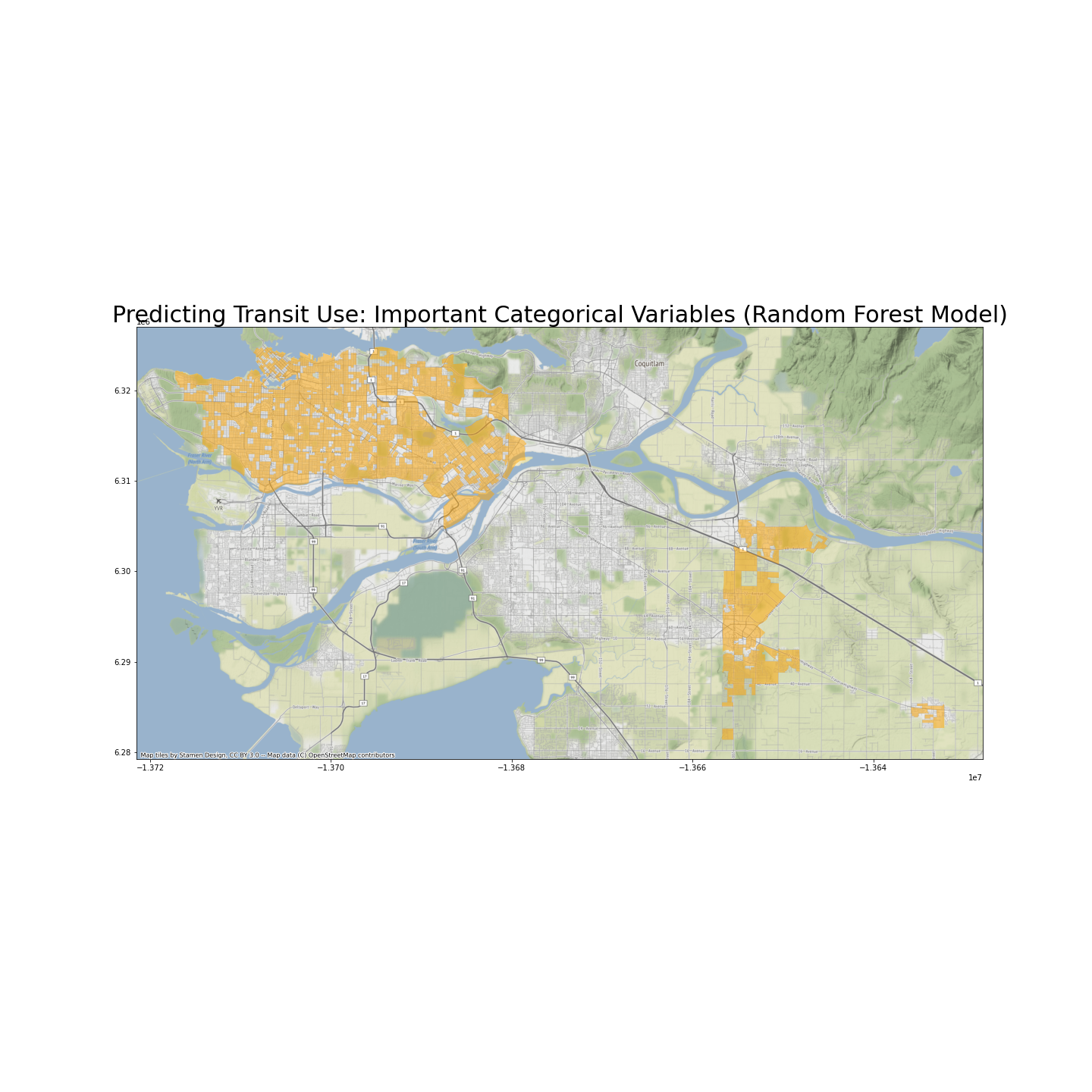
If I can make a guess, however, areas in the city of Vancouver probably tend to have higher rates of transit use. By contrast, The east part of Langley city and Aldergrove probably have low transit use. We will know more details about each feature’s impact later using SHAP.
Numeric features
LASSO model
| coeffs | explanation | |
|---|---|---|
| 620 | 0.022032 | Immigration - Total Sex / Total - Age at immigration for the immigrant population in private households - 25% sample data / 25 to 44 years |
| 711 | 0.021731 | Labour - Total Sex / Participation rate |
| 383 | 0.018865 | Households - Both sexes / Total - Persons not in census families in private households - 100% data ; Both sexes |
| 682 | 0.016852 | Ethnic Origin - Total Sex / Total - Ethnic origin for the population in private households - 25% sample data / European origins / British Isles origins |
| 439 | 0.016713 | Housing - Total Sex / Total - Owner and tenant households with household total income greater than zero, in non-farm, non-reserve private dwellings by shelter-cost-to-income ratio - 25% sample data / Spending less than 30% of income on shelter costs |
As shown in the table above, important numeric factors that indicate high transit use include:
(1) Large number of immigrant population who moved to Canada when they were 25 to 44 years old,
(2) High labor participation rate (number of people working as a percentage of total population),
(3) High number of people who do not live in families,
(4) High number of people of British ethnicity, and
(5) High number of people who spend less money on housing as compared to their income.
| coeffs | explanation | |
|---|---|---|
| 712 | -0.016735 | Labour - Total Sex / Employment rate |
| 724 | -0.015868 | Labour - Total Sex / Total labour force aged 15 years and over by class of worker - 25% sample data / All classes of workers / Self-employed |
| 790 | -0.014384 | Journey to Work - Males / Total - Commuting destination for the employed labour force aged 15 years and over in private households with a usual place of work - 25% sample data / Commute within census subdivision (CSD) of residence |
| 448 | -0.013827 | Housing - Total Sex / Total - Owner households in non-farm, non-reserve private dwellings - 25% sample data / Average value of dwellings ($) |
| 453 | -0.013343 | Housing - Total Sex / Total - Tenant households in non-farm, non-reserve private dwellings - 25% sample data / Average monthly shelter costs for rented dwellings ($) |
As shown in the table above, the following numeric features most strongly predict low transit use:
(1) High employment rate (number of people actually employed as a percentage of people who want to be employed),
(2) Large self-employed population,
(3) Large number of people working in the same CSD,
(4) High average value of dwellings, and
(5) High average housing cost for rented dwellings.
We are also interested in knowing where the two transit access variables are ranked among the numeric features. It turns out that among 462 numeric features, number of services per capita ranks 20, coefficient is 0.0060. However, the number of stops per capita has zero coefficient.
Random Forest model
| impurity_importance | explanation | |
|---|---|---|
| 349 | 0.036776 | Population and dwelling counts / Population density per square kilometre |
| 800 | 0.019114 | NBA_services_PC |
| 548 | 0.006549 | Income - Total Sex / Total - Income statistics in 2015 for the population aged 15 years and over in private households - 100% data / Number of government transfers recipients aged 15 years and over in private households - 100% data / Median government transfers in 2015 among recipients ($) |
| 352 | 0.004274 | Dwelling characteristics / Total - Occupied private dwellings by structural type of dwelling - 100% data / Single-detached house |
| 415 | 0.003868 | Housing - Total Sex / Total - Occupied private dwellings by period of construction - 25% sample data / 1960 or before |
The table above show the important numeric features in our Random Forest model. Population density turns out to be the most important one. Also, much to our pleasant surprise, number of services per capita, the variable that we are interested in, ranks the second.
Other important features include high amounts of government transfer recipients, high number of single-detached house, and very old house dwellings.
Proportional features
LASSO model
| coeffs | Explanation | |
|---|---|---|
| 1336 | 0.047517 | Denominator is Labour - Total Sex / Total labour force population aged 15 years and over by occupation - National Occupational Classification (NOC) 2016 - 25% sample data / All occupations; numerator is Labour - Total Sex / Total labour force population aged 15 years and over by occupation - National Occupational Classification (NOC) 2016 - 25% sample data / All occupations / 6 Sales and service occupations. |
| 1156 | 0.046837 | Denominator is Labour - Total Sex / Total - Place of work status for the employed labour force aged 15 years and over in private households - 25% sample data; numerator is Labour - Total Sex / Total - Place of work status for the employed labour force aged 15 years and over in private households - 25% sample data / Worked at usual place. |
| 1097 | 0.044393 | Denominator is Ethnic Origin - Total Sex / Total - Ethnic origin for the population in private households - 25% sample data; numerator is Ethnic Origin - Total Sex / Total - Ethnic origin for the population in private households - 25% sample data / Asian origins / East and Southeast Asian origins. |
| 1182 | 0.040103 | Denominator is Journey to Work - Females / Total - Commuting destination for the employed labour force aged 15 years and over in private households with a usual place of work - 25% sample data; numerator is Journey to Work - Females / Total - Commuting destination for the employed labour force aged 15 years and over in private households with a usual place of work - 25% sample data / Commute to a different census subdivision (CSD) within census division (CD) of residence. |
| 821 | 0.037006 | Denominator is Family characteristics / Total - Couple census families in private households - 100% data; numerator is Family characteristics / Total - Couple census families in private households - 100% data / Couples with children. |
As shown in the table above, strong predictors for high transit use, among proportion variables, include:
(1) High proportion of people working in sales and service industries,
(2) High proportion of people working at a constant and usual location,
(3) High proportion of people with East and Southeast Asian ethnic origins,
(4) High proportion of people commuting to a different CSD but the same CD for work, and
(5) High proportion of households that have couples with children.
| coeffs | explanation | |
|---|---|---|
| 829 | -0.046500 | Denominator is Housing - Total Sex / Total - Private households by tenure - 25% sample data; numerator is Housing - Total Sex / Total - Private households by tenure - 25% sample data / Owner. |
| 1055 | -0.026167 | Denominator is Immigration - Total Sex / Total - Generation status for the population in private households - 25% sample data; numerator is Immigration - Total Sex / Total - Generation status for the population in private households - 25% sample data / Third generation or more. |
| 1289 | -0.023855 | Denominator is Immigration - Total Sex / Total - Selected places of birth for the immigrant population in private households - 25% sample data / Asia; numerator is Immigration - Total Sex / Total - Selected places of birth for the immigrant population in private households - 25% sample data / Asia / India. |
| 878 | -0.014456 | Denominator is Housing - Total Sex / Total - Tenant households in non-farm, non-reserve private dwellings - 25% sample data; numerator is Housing - Total Sex / Total - Tenant households in non-farm, non-reserve private dwellings - 25% sample data / % of tenant households spending 30% or more of its income on shelter costs. |
| 1368 | -0.010210 | Denominator is Mobility - Total Sex / Total - Mobility status 5 years ago - 25% sample data / Movers / Migrants; numerator is Mobility - Total Sex / Total - Mobility status 5 years ago - 25% sample data / Movers / Migrants / Internal migrants. |
By contrast, strong predictors for low transit use, among proportion variables, include:
(1) High proportion of people who live in a dwelling which they own,
(2) High proportion of households where three or more generations live together,
(3) High number of immigrants who are born in India, as a proportion of all immigrants born in Asia,
(4) High proportion of tenant households spending 30% or more of its income on shelter costs, and
(5) High number of internal migrants as a proportion of all migrants.
Random forest model
| impurity_importance | explanation | |
|---|---|---|
| 813 | 0.281665 | Denominator is Marital Status - Both Sexes / Total - Marital status for the population aged 15 years and over - 100% data ; Both sexes; numerator is Marital Status - Both Sexes / Total - Marital status for the population aged 15 years and over - 100% data ; Both sexes / Married or living common law ; Both sexes. |
| 814 | 0.034743 | Denominator is Marital Status - Both Sexes / Total - Marital status for the population aged 15 years and over - 100% data ; Both sexes; numerator is Marital Status - Both Sexes / Total - Marital status for the population aged 15 years and over - 100% data ; Both sexes / Not married and not living common law ; Both sexes. |
| 1097 | 0.034705 | Denominator is Ethnic Origin - Total Sex / Total - Ethnic origin for the population in private households - 25% sample data; numerator is Ethnic Origin - Total Sex / Total - Ethnic origin for the population in private households - 25% sample data / Asian origins / East and Southeast Asian origins. |
| 958 | 0.030017 | Denominator is Other language spoken regularly at home - Both sexes / Total - Other language(s) spoken regularly at home for the total population excluding institutional residents - 100% data ; Both sexes; numerator is Other language spoken regularly at home - Both sexes / Total - Other language(s) spoken regularly at home for the total population excluding institutional residents - 100% data ; Both sexes / Non-official language ; Both sexes. |
| 955 | 0.028454 | Denominator is Other language spoken regularly at home - Both sexes / Total - Other language(s) spoken regularly at home for the total population excluding institutional residents - 100% data ; Both sexes; numerator is Other language spoken regularly at home - Both sexes / Total - Other language(s) spoken regularly at home for the total population excluding institutional residents - 100% data ; Both sexes / None ; Both sexes. |
In our Random Forest model, marital status of residents have the most impact on use of public transit. Other important proportional features include:
(1) Number of immigrants from East and Southeast Asia as a proportion of all immigrants,
(2) Proportion of residents speaking more than two languages at home, with the second language not being an official language.
(3) Proportion of residents who only speak one language at home.
SHAP analyses on Random Forest model
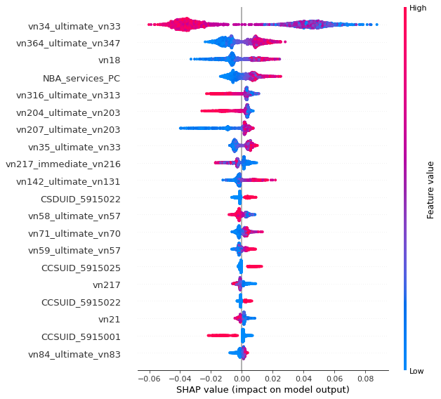
Here, we use the SHapley Additive exPlanations (SHAP) tool to further understand the effects of features in our Random Forest model.
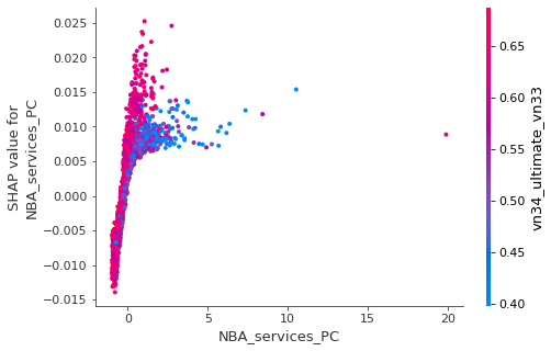
The variable that we are most interested in, of course, is number of services per capita in the neighborhood area NBA_services_PC. Two takeaways are worth of mentioning here:
(1) The relationship between NBA_services_PC and transit use is positive, with the only exception of very large NBA_services_PC values.
(2) Among other variables, vn34_ultimate_vn33 (proportion of married or common-law couples among all residents) has highest frequency of interaction with NBA_services_PC. The relationship between NBA_services_PC and transit use seems to be more positive for areas with high proportions of married people.
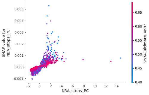
Another variable that we are interested in is NBA_stops_PC, the number of stops in the neighborhood area. As we can see in the following plot, it also has a positive, albeit weaker relationship with transit use. Also interestingly, there seems to be a strong interaction between NBA_stops_PC and vn142_ultimate_vn131, which is the proportion of people who speak an non-official language as their mother tongue. For DAs with more presence of such population, the relationship between transit stops and public transportation use seems stronger.
To gain an understanding of all key features that impact transit use at the DA level, please see the charts below.
Summary
We have not figured out where GVA’s public transportation agency should prioritize in terms of service and infrastructure development yet. However, the analyses above provide valuable information about the relationship between demographic characters and transit use in GVA, especially the role of access to public transportation services and stops.
Geographically speaking, areas in and around the downtown core tend have higher public transit use, something hardly surprising given our prior analyses on the spatial distribution of transit services in the area. However, variations within the downtown core should not be overlooked.
In addition to geographical location, factors that impact transit use are diverse, seen across most demographic aspects covered by the census. DA level variables in ethnicity, family structure, housing, immigration, labor and language all make to the top of importance.
Access to transit does seem to affect people’s transit use, with all other variables above taken into consideration. Both our models agree that number of services per capita in a DA’s neighborhood area is a more important feature than the number of stops per capita. Our LASSO model does not even give the number of stops per capita a non-zero coefficient. This seems to suggest that the authority should pour more of their resources into strengthening transit services at existing locations, instead of setting up new stops.
Exactly how important are transit services and stops? In fact, the two models diverge to a certain degree. What we can be confident about for now, however, is that number of transit services per capita is among the 5% most important numeric features, and is related to transit use positively.
Policy recommendations
How should our analyses inform decision makers? In the last section of this project, I will bring back the whole dataset and identify areas that GVA’s transportation agency should pour its resources to. Bearing in mind that the government’s resources are limited and come from tax payers’ money, we should assume that it can only increase access to transit for a limited number of neighborhoods. Therefore, the selected neighborhoods should be places where the same increase in transit access lead to the most increase in proportion of people using transit, which is defined as the following:
increase in proportion of people using transit = proportion of people using transit as predicted by the model, after increase in transit access - current proportion of people using transit as predicted by the model
Two scenarios
I will specify two scenarios in which access to public transit services increases.
Scenario 1
(1) I will create a hypothetical dataset (X_1) where each DA’s NBA_services_PC increases by a fixed amount (10% of average current NBA_services_PC across all DAs in GVA, or about 1.2 percentage points). I will then identify DAs where transit use rate increases the most, measured by percentage point increase.
The following two maps identify DAs with top 10% percentage point increase in transit use if number of transit services per person increases by about 1.2 in the neighborhood area.
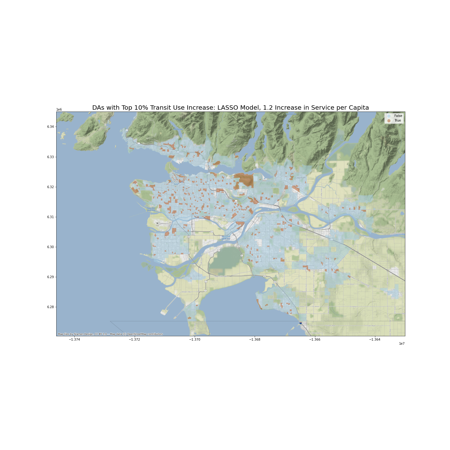

Are our predictions of increase in transit use similar between the two models? I have calculated the Pearson correlation coefficient between two sets of predictions, which stands at 0.768. This result is satisfactory.
Scenario 2
(2) I will create a hypothetical dataset (X_2) where each DA’s NBA_services_PC increases by a fixed percentage (10%) of current NBA_services_PC. I will then identify as a percentage of current transit use rate increases the most, measured by percentage increase.
The following two maps identify DAs with top 10% percentage point increase in transit use if number of transit services per person increases by 10 percent of the current value, in the neighborhood area.
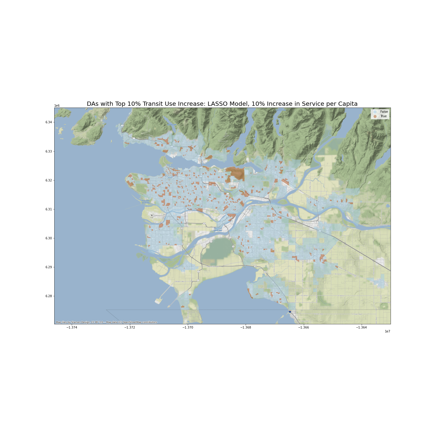

The two models’ predictions, under scenario 2, are also quite similar. I have calculated the Pearson correlation coefficient between two sets of predictions, which stands at 0.767.
Impact evaluation
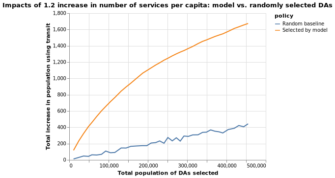
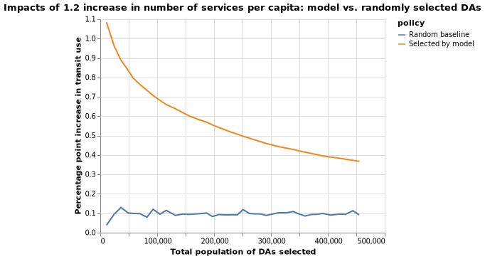
If the public transportation authority of GVA does indeed increase service in the key areas, how much increase of transit use can we expect? A more fundamental question is that, although increase in access to public transit does have a positive impact on use of transit in commuting, how many DAs in GVA should be prioritized? The following analyses show that the law of diminishing returns hold here, and the more DAs we target, the less increase in transit use we will see. However, as compared to the baseline scenario where we increase transit services in randomly selected DAs, a policy based on our models still results in far more increase in overall transit use in GVA overall.
I want to point out that here, only the Random Forest model, instead of the LASSO model, is used in the calculations. This is because LASSO is essentially a linear model, and a fixed increase in access to transit will result in the same increase in transit usage, which is not useful in selecting DAs to prioritize.
Scenario 1
The following charts show that as compared to the baseline, a policy to increase transit access informed by our model does result in more increase in public transportation use. For example, if we target DAs with a combined population of 100,000 and increase their number of transit services per capita by 1.2, we are expected to see 0.7 percentage point increase in proportion of people using transit, which translates into 700 more people using transit. By contrast, if we randomly select DAs also with a combined population of 100,000, we are only expected to see 100 more people using transit. If we target DAs with a combined population of 400,000 and and increase their number of transit services per capita by 1.2, we are expected to see 0.4 percentage point increase in proportion of people using transit, which translates into 1600 more people using transit. By contrast, if we randomly select DAs also with a combined population of 400,000, we are only expected to see 400 more people using transit.
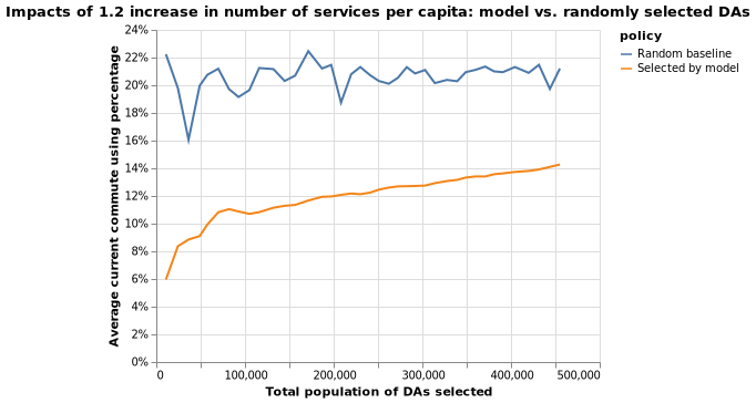
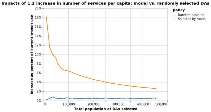
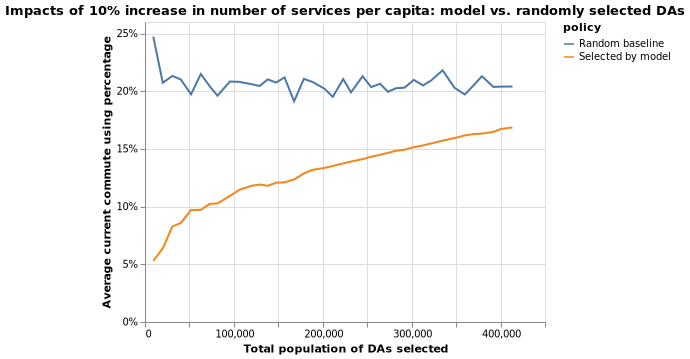
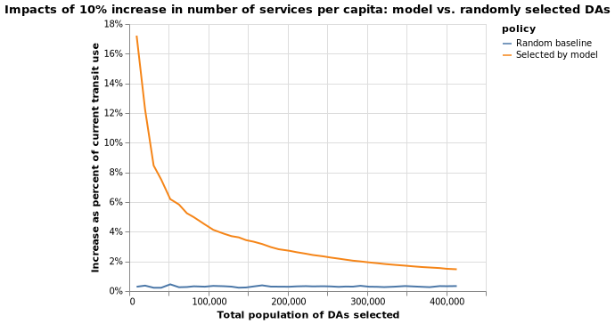
The following two charts put the impact of the policy specified above into context. For example, if we target DAs with a combined population of 200,000, they in average have 12% people commutting using public transit at present. After the policy intervention, the percentage of people using public transit will increase by 0.55 percentage points, or about 5%.
Scenario 2
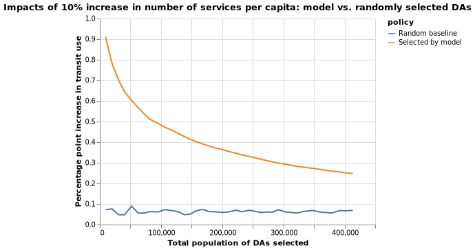
Simulation results for scenario 2 are similar, as shown below.

Discussion
These results should be taken with a grain of salt.
It is unrealistic to expect that some infrastructure development will only increase service in selected DAs while keeping service in other DAs constant. This point has two implications. On the one hand, even the transit authority focuses solely on increasing service in identified areas, other areas across GVA will benefit. On the other hand, a “increasing service by 10% in 10% of all DAs” scenario does not mean that the system’s variable cost will increase by 1% (10% * 10%). Most likely, the real cost increase will be significantly bigger.
In addition, our model only takes into account a limited number of factors, and there are certainly importrant variables which would help to build our predictive models, but we do not have data for. For example, we do not know whether public transportation has been in a DA long enough for people there to have a habit of using transit.
Lastly, there is this fundamental problem of applying inference models to prediction. Without randomized trials, which seems extremely expensive in our case, we cannot know for sure whether the seemlying strong relationship between access to transit service and transit use is causal. Therefore, when we pour resourse into these areas, the outcome may not be as strong as what we might expect.
